Track Generation
To create a track, use the script
crs/src/tools/track_generation/src/simple_track_generator.py
Generating the default track
Running the script, without changing it, will generate the demo track by default. The plot, which will be generated, will look as follows:
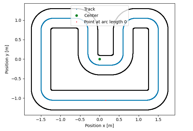
Command line output:
x_init: 0.15000000000000002
y_init: -1.04999999999999994
yaw_init: 0.0
Total Arc Length: 11.568244517641709
Created information
The track is saved to the track.yaml file in the track_generation package. The following track properties are stored in this yaml file:
| name | description |
|---|---|
| xCoords | array containing the x coordinates of all points on track centerline |
| yCoords | array containing the y coordinates of all points on track centerline |
| xRate | array containing the rate of change in x direction of all points on track centerline |
| yRate | array containing the rate of change in y direction of all points on track centerline |
| tangentAngle | array containing the tangent angle of the track at this index |
| arcLength | array containing the distance on the centerline from the start to this index |
| curvature | array containing the curvature (1/radius, zero if straight) at of the track segment from the start to this index |
| trackWidth | width of the track |
| x_init | initial x position of car on this track |
| y_init | initial y position of car on this track |
| yaw_init | initial orientation of car on this track |
Careful! Note that the track saved in the track.yaml file goes twice around! This means that every point on the track exists twice.
Varying the track density and the track width
The constructor of the track generator takes two arguments: the track density and the track width.
An example of a lower density track:
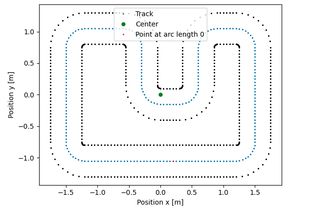
Careful! The default density has proven to be good. It is unlikely, that it needs to be changed.
An example of a thinner track:
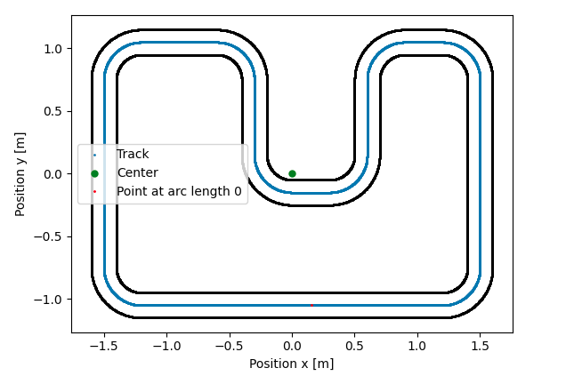
Careful! When you change the track width, the constraint for the track width in MPCC needs to be changed manually at the moment. The file containing the constraint can be found in the forces_control_generation of the MPCC variant in use, and is called either mpcc_formulation_pacejka.m, or mpcc_formulation_pacejka_RK4.m, depending on the discretization method being used.
Similarly, the track width needs to be changed in the visualizer node configuration file. The file is called car_track_visualizer.yaml.
Creating your own track
The track generator currently chains straight line segments and arc segments together, as specified by the user. To create your first track, you need to choose a starting point and a starting orientation as follows:
init = [0,0,0]
Additionally, it is very useful, to define a "tile size". The tile size can be interpreted as a scaling factor for the track. So far a tile size of t=0.3 has been the most common choice, since the Kyosho tiles have exactly this length.
As an example, we will start with a straight segment, that is 2 tiles long, and chain a 180° degree left turn with a two tile radius to it. Then we add another 2 tile straight and finish the track by adding another two-tile-radius arc of 180°:
t = 0.3 # tile length
init = [0, 0, 0]
next = gen.straight(init, 2*t)
next = gen.left_turn(next, 2*t, np.pi)
next = gen.straight(next, 2*t)
next = gen.left_turn(next, 2*t, np.pi)
Resulting Image:
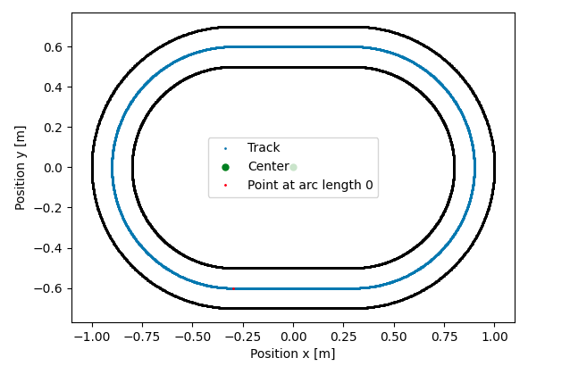
Command Line Output:
The track is always centered after generating it, shifting the starting point to a different location. The initial condition of the car needs to be updated, whenever a new track is generated. The initial condition for the ros framework can found in the file src/model/car/pacejka_model/config/pacejka_model.yaml. The snippet to be changed, looks as follows:
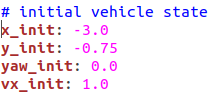
Only x_init, y_init and yaw_init need to be changed to match command line output of the script. In this case, they need to be changed to -0.3, -0.6 and 0.0, respectively.
Track examples
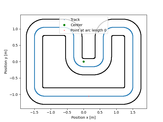
Demo Track
t = 0.3
init = [0,0,0]
next = gen.straight(init, 3.5*t)
next = gen.left_turn(next,t,np.pi/2)
next = gen.straight(next, 5*t)
next = gen.left_turn(next,t,np.pi/2)
next = gen.straight(next, 1*t)
next = gen.left_turn(next,t,np.pi/2)
next = gen.straight(next, 2*t)
next = gen.right_turn(next,t,np.pi/2)
next = gen.straight(next, 1*t)
next = gen.right_turn(next,t,np.pi/2)
next = gen.straight(next, 2*t)
next = gen.left_turn(next,t,np.pi/2)
next = gen.straight(next, 2*t)
next = gen.left_turn(next,t,np.pi/2)
next = gen.straight(next, 5*t)
next = gen.left_turn(next,t,np.pi/2)
next = gen.straight(next, 4.5*t)
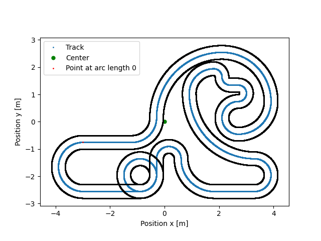
Hard Track
    next = gen.straight(init,6*t)
    next = gen.left_turn(next, 3*t, np.pi/2)
    next = gen.right_turn(next,8*t, np.pi/2)
    next = gen.right_turn(next, 6*t, np.pi/2)
    next = gen.right_turn(next, 4*t, np.pi/2)
    next = gen.right_turn(next, 2*t, np.pi)
    next = gen.left_turn(next, 1*t, np.pi)
    next = gen.straight(next, 1*t)
    next = gen.right_turn(next, 1*t, np.pi/2)
    next = gen.left_turn(next, 1*t, np.pi/2)
    next = gen.left_turn(next, 3*t, np.pi/2)
    next = gen.left_turn(next, 8*t, np.pi/2)
    next = gen.right_turn(next, 2*t, np.pi)
    next = gen.straight(next, 5*t)
    next = gen.right_turn(next, 4*t, np.pi/2)
    next = gen.left_turn(next, 1.5*t, np.pi)
    next = gen.straight(next, 2*t)
    next = gen.right_turn(next, 2*t, 2.5*np.pi)
    next = gen.straight(next, 7*t)
    next = gen.right_turn(next, 3*t, np.pi)
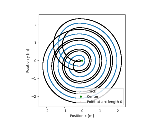
Snail Track
    next = gen.left_turn(init,t,np.pi)
    for i in range(6):
        next = gen.left_turn(next,(i+2)*t,np.pi)

    next = gen.left_turn(next,4*t,np.pi)
Analytical Curvature
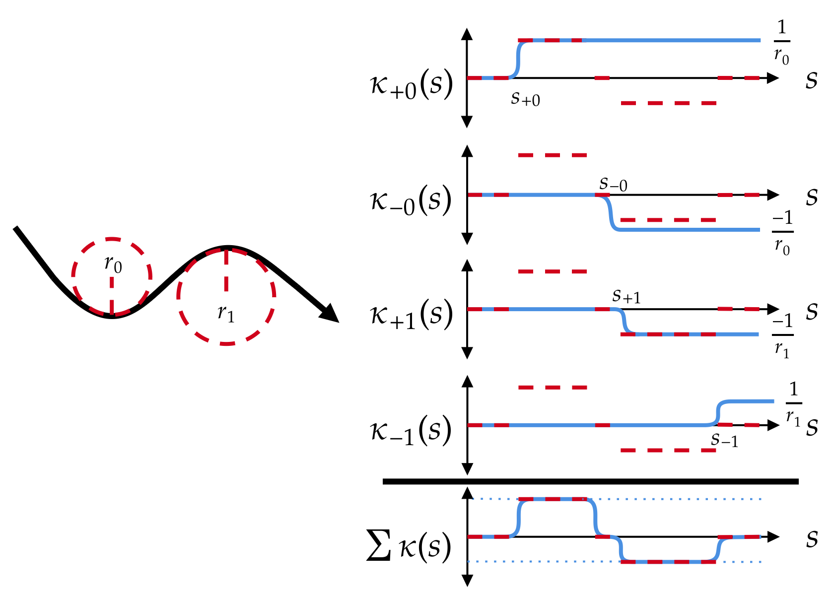
The file analytical_curvature.py contains the function fit_sigmoids_to_curvature which was originally formulated by Jelena Trisovic and later integrated and tested in CRS-2.0 by Justin Shim.
Given an arbitrary racetrack, we assume we are given the finite sets \(X_t, Y_t\), which comprise of the Cartesian coordinates of the racetrack's centerline measured at discrete points. Furthermore, we also assume we have access to \(\Kappa_t\), which comprise of the track curvature at each discrete point. Prior to the addtion of analytical_curvature.py, this data was already provided by the existing functions in simple_track_generator.py.
Generally speaking, the curvature at a point \(s\), where \(s\) is the arc length (curvilinear abscissa) from the beginning of the track, is \(1/r\), where \(r\) is the radius of the circle whose circumference matches the arc length of the track around \(s\). For example, a sharp turn will have a larger curvature than a more gentle turn, and a straight section of track will have a curvature of \(0\) because the circle that describes its arc length is infinitely large.
Furthermore, an arbitrary racetrack can be decomposed into \(N\) distinct sections of constant curvature. Thus, any single curve or turn can be modelled as the two distinct changes in curvature-- one at the beginning and the second at the end of the curve. As shown above, the track curvature in the \(i^{th}\) section between \(s_{i}\) and \(s_{i+1}\), where \(s_i, s_{i+1}\) describe where the section begins and ends, respectively, can be modeled as the sum of the sigmoid functions
where \(\sigma\) is a parameter that controls the steepness of the change in curvature 1.
Example
Below, you can find an example implementation of reading in the generated parameters to define a casadi function that evaluates the curvature at the current progress (i.e., arc length) of the vehicle state.
casadi::MX getAnalyticalTrackCurvature(const casadi::MX progress)
{
  using namespace casadi;
  auto kappa = casadi::MX::zeros();

  auto sigma = trajectory->getSigma();
  std::vector<double> sigmoid_parameters = trajectory->getSigmoidParameters();

  size_t num_turns = static_cast<size_t>(sigmoid_parameters.size() / 3);

  for (size_t i = 0; i < num_turns; i++)
  {
    double a = sigmoid_parameters[3 * i];
    double b = sigmoid_parameters[(3 * i) + 1];
    double c = sigmoid_parameters[(3 * i) + 2];
    kappa += a + (c / (1 + exp(-sigma * (progress - b))));
  }

  return kappa;
}
-
Note that \(\sigma\) is set to a default value of \(67\) as large values of \(\sigma\) have resulted in solver issues. ↩