MPCC
MPCC is an optimal control approach. In each control iteration, the controller will compute thebest feasible trajectory for the car within a certain time horizon, starting at the current car's state. It then applies only the first control input that would lead to this optimal trajectory and repeat the whole process over and over again.
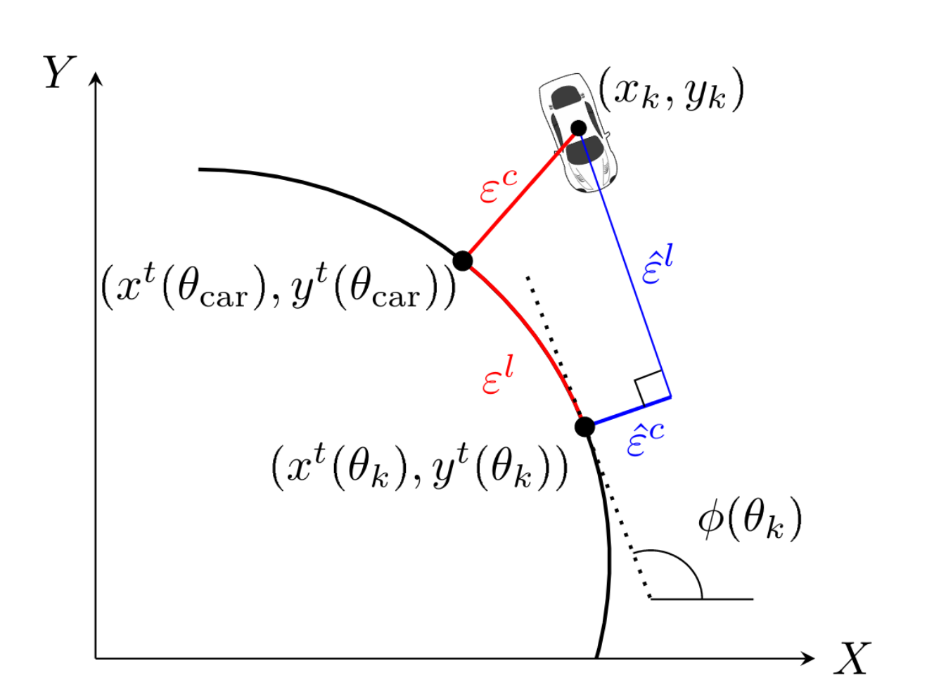
The cost that MPCC is minimizing consists of several terms. The first term is the contouring error εc. This is the lateral distance between the car and the track. The second term is the lag error εl. This is the distance on the centerline between the current car's position and the "desired" car's position θ. The θ is part of the optimization problem itself and has a negative influence on the cost. This means that the controller tries to find θ that is as advanced as possible, while at the same time penalizing the lag behind that θ. Last, the change in steer and torque is also contributing to the cost to guarantee smoothness.
Since it is not tractable to compute εc and εl directly (red in figure below), they need to be approximated (blue in figure below).
To compute the vehicle's trajectory, it needs a car model and is therefore model-dependent. It can either use the kinematic or the pacejka vehicle model.
Solvers
In an implementation, an MPCC controller needs an efficient solver that can give a solution to this optimization problem in a few milliseconds.
Available Solvers
Building Solvers
-
Acados:
The Nominal MPC controller uses the pacejka vehicle model in combination with the solver Acados. In order to build the solver, you need to go to the directoryroscd acados_pacejka_solverand execute./script/create_solver.sh. -
FORCESPRO:
In order to build the forces solver you will need to have access to a license. Step-by-step instructions on how to generate the solver using a proxy server is given here: FORCESPRO Solver
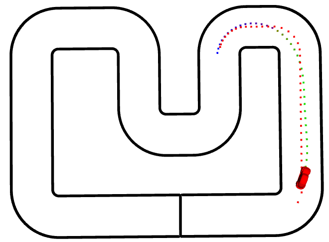 _View of the RVIZ visualizer of the CRS demo track and car using the mpc controller_
 The $\textcolor{red}{\text{red}}$ trajectory shows reference points sampled of the center line used for the mpc path planning. The other trajectory denotes the planned mpc trajectory with the respective speed color coded. Low speeds are colored $\textcolor{blue}{\text{blue}}$ and high speeds are colored $\textcolor{green}{\text{green}}$ |
Updating sampling time / Horizon Length
If you want to change the control horizon N, you cannot do this by only modifying the config file. You need to change this in <acados_control_generation>/script/generate_acados_solver.py and then rerun the generator script. This will modify N, npar and nvar in the config file by itself. You will also need to update the values in the <acados_control_generation>/src/pacejka_solver.cpp by changing the value of the getHorizonLength() function
Full Yaml Config Structure
car_track_visualizer.yaml
state_type: pacejka_car
input_type: pacejka_car

controller_type: MPCC
max_rate: 30

controller_params:
  Q1: 100.0
  Q2: 200.0
  R1: 0.2
  R2: 0.3
  R3: 0.2
  q: 3.5
  lag_compensation_time: 0.01 #
  solver_type: ACADOS


# model: # Model specific parameters. Must not be complete.
model_params: # only missmatch mass and Intertia
  # size params
  # lr: 0.038
  # lf: 0.052
  m: 0.200
  # I: 0.000505

  # lateral force params
  # Df: 0.65
  # Cf: 1.5
  # Bf: 5.2
  # Dr: 1.0
  # Cr: 1.45
  # Br: 8.5

  # longitudinal force params
  # Cm1: 0.98028992
  # Cm2: 0.01814131
  # Cd: 0.02750696
  # Croll: 0.08518052


# Visualization parameters for mpc visualizer
visualizer:
  type: mpc
  rate: 10

  # Visualizer specific  parameters
  frame_id: crs_frame # default
  namespace: mpc # default

  use_arrows: false # If true, use arrows to visualize planned and reference yaw angle. This option is a lot slower and may introduce visual lags

  double_min_velocity: 1.5 # Min velocity for visualization (this or below gets mapped to blue)
  double_max_velocity: 2.5 # Max velocity for visualization (this or above gets mapped to red)

  planned: # marker size of planned trajectory
    size_x: 0.02 # 0.07 for arrows
    size_y: 0.02 # 0.02 for arrows
    size_z: 0.02 # 0.02 for arrows

  reference: # marker size and color of reference trajectory
    r: 1
    g: 0
    b: 0
    a: 1
    size_x: 0.02 # 0.07 for arrows
    size_y: 0.02 # 0.02 for arrows
    size_z: 0.02 # 0.02 for arrows