Pacejka Model
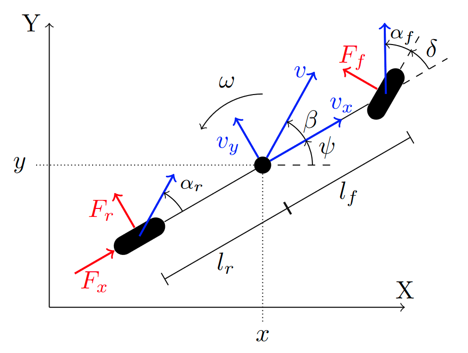
The Pacejka model is a more realistic depiction of reality compared to the kinematic car model. It also models the vehicle's dynamics including several contact forces, most prominently from tire slip.
The front and rear tire forces are modeled by the Pacejka Magic Formula, which gives it its name. The drivetrain is also modeled dynamically and no longer simplified to a first order system. This is why the input torque no longer has the physical meaning of the steady state velocity but is just a number in the range of 0 and 1. In contrast to the kinematic model it also has much more model parameters that need to be estimated.
Model Dynamics
The motor generates a force \(F_{\mathrm m}\) that is distributed among the front and rear axle, parametrized by the torque split parameter \(\gamma\) (for \(\gamma = 0.5\) we have an all-wheel-drive vehicle, and for \(\gamma = 1\) a real-wheel-drive). The friction force is modeled as a Taylor expansion in \(\dot x\) and affects the longitudinal velocity directly.
The slip angles are computed as
where \(\epsilon\) is a parameter that can be set and determines at which velocity the slip angle computation switches. The coefficients \(b_f, c_f, b_r, c_r\) are given as
Parameter Information
| Parameters | Description |
|---|---|
| Bf | Front tire stiffness factor |
| Br | Rear tire stiffness factor |
| Cd0 | Friction expansion 0th order coefficient |
| Cd1 | Friction expansion 1st order coefficient |
| Cd2 | Friction expansion 2nd order coefficient |
| Cf | Front tire shape factor that controls the ‘stretching’ in the x direction |
| Cm1 | Model parameter |
| Cm2 | Model parameter |
| Cr | Rear tire shape factor that controls the ‘stretching’ in the x direction |
| Df | Peak value for front tire. |
| Dr | Peak value for rear tire. |
| I | Inertia |
| lf | Length from center to front wheel |
| lr | Length from center to rear wheel |
| m | Mass of car |
| \(\gamma\) | Torque split between front and rear axle |
| \(\epsilon\) | Velocity at which the approximated slip angles are used to avoid singularities at zero velocity |
Configuration
type: "pacejka_discrete"

# Q (process noise covariance matrix)
Q:
  value:
    [
      [0.001, 0, 0, 0, 0, 0],
      [0, 0.001, 0, 0, 0, 0],
      [0, 0, 0.001, 0, 0, 0],
      [0, 0, 0, 0.01, 0, 0],
      [0, 0, 0, 0, 0.01, 0],
      [0, 0, 0, 0, 0, 0.001],
    ]
  is_diag: false

model_params:
  # size params
  lr: 0.038
  lf: 0.052
  m: 0.201
  I: 0.000705

  wheel_radius: 0.0175
  car_width: 0.12

  # lateral force params
  Df: 0.65
  Cf: 1.5
  Bf: 5.2
  Dr: 1.0
  Cr: 1.45
  Br: 8.5

  # longitudinal force params
  Cm1: 0.98028992
  Cm2: 0.01814131

  # friction force params
  Cd0: 0.08518052
  Cd1: 0.01
  Cd2: 0.02750696

  tau: 0.1 # to make this compatible with kinematic model
  eps: 0.2 # determines at what velocity we switch from atan to the polynomial approximation of arctan(w/x)
  gamma: 0.5